Spatial Transformer Networks Tutorial

Created On: Nov 08, 2017 | Last Updated: Jan 19, 2024 | Last Verified: Nov 05, 2024

Author: Ghassen HAMROUNI

In this tutorial, you will learn how to augment your network using a visual attention mechanism called spatial transformer networks. You can read more about the spatial transformer networks in the DeepMind paper

Spatial transformer networks are a generalization of differentiable attention to any spatial transformation. Spatial transformer networks (STN for short) allow a neural network to learn how to perform spatial transformations on the input image in order to enhance the geometric invariance of the model. For example, it can crop a region of interest, scale and correct the orientation of an image. It can be a useful mechanism because CNNs are not invariant to rotation and scale and more general affine transformations.

One of the best things about STN is the ability to simply plug it into any existing CNN with very little modification.

# License: BSD
# Author: Ghassen Hamrouni

import torch
import torch.nn as nn
import torch.nn.functional as F
import torch.optim as optim
import torchvision
from torchvision import datasets, transforms
import matplotlib.pyplot as plt
import numpy as np

plt.ion()   # interactive mode

<contextlib.ExitStack object at 0x7f69cf06c9d0>

Loading the data

In this post we experiment with the classic MNIST dataset. Using a standard convolutional network augmented with a spatial transformer network.

from six.moves import urllib
opener = urllib.request.build_opener()
opener.addheaders = [('User-agent', 'Mozilla/5.0')]
urllib.request.install_opener(opener)

device = torch.device("cuda" if torch.cuda.is_available() else "cpu")

# Training dataset
train_loader = torch.utils.data.DataLoader(
    datasets.MNIST(root='.', train=True, download=True,
                   transform=transforms.Compose([
                       transforms.ToTensor(),
                       transforms.Normalize((0.1307,), (0.3081,))
                   ])), batch_size=64, shuffle=True, num_workers=4)
# Test dataset
test_loader = torch.utils.data.DataLoader(
    datasets.MNIST(root='.', train=False, transform=transforms.Compose([
        transforms.ToTensor(),
        transforms.Normalize((0.1307,), (0.3081,))
    ])), batch_size=64, shuffle=True, num_workers=4)

  0%|          | 0.00/9.91M [00:00<?, ?B/s]
100%|##########| 9.91M/9.91M [00:00<00:00, 203MB/s]

  0%|          | 0.00/28.9k [00:00<?, ?B/s]
100%|##########| 28.9k/28.9k [00:00<00:00, 34.7MB/s]

  0%|          | 0.00/1.65M [00:00<?, ?B/s]
100%|##########| 1.65M/1.65M [00:00<00:00, 171MB/s]

  0%|          | 0.00/4.54k [00:00<?, ?B/s]
100%|##########| 4.54k/4.54k [00:00<00:00, 27.8MB/s]

Depicting spatial transformer networks

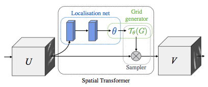
Spatial transformer networks boils down to three main components :

• The localization network is a regular CNN which regresses the transformation parameters. The transformation is never learned explicitly from this dataset, instead the network learns automatically the spatial transformations that enhances the global accuracy.

• The grid generator generates a grid of coordinates in the input image corresponding to each pixel from the output image.

• The sampler uses the parameters of the transformation and applies it to the input image.

Note

We need the latest version of PyTorch that contains affine_grid and grid_sample modules.

class Net(nn.Module):
    def __init__(self):
        super(Net, self).__init__()
        self.conv1 = nn.Conv2d(1, 10, kernel_size=5)
        self.conv2 = nn.Conv2d(10, 20, kernel_size=5)
        self.conv2_drop = nn.Dropout2d()
        self.fc1 = nn.Linear(320, 50)
        self.fc2 = nn.Linear(50, 10)

        # Spatial transformer localization-network
        self.localization = nn.Sequential(
            nn.Conv2d(1, 8, kernel_size=7),
            nn.MaxPool2d(2, stride=2),
            nn.ReLU(True),
            nn.Conv2d(8, 10, kernel_size=5),
            nn.MaxPool2d(2, stride=2),
            nn.ReLU(True)
        )

        # Regressor for the 3 * 2 affine matrix
        self.fc_loc = nn.Sequential(
            nn.Linear(10 * 3 * 3, 32),
            nn.ReLU(True),
            nn.Linear(32, 3 * 2)
        )

        # Initialize the weights/bias with identity transformation
        self.fc_loc[2].weight.data.zero_()
        self.fc_loc[2].bias.data.copy_(torch.tensor([1, 0, 0, 0, 1, 0], dtype=torch.float))

    # Spatial transformer network forward function
    def stn(self, x):
        xs = self.localization(x)
        xs = xs.view(-1, 10 * 3 * 3)
        theta = self.fc_loc(xs)
        theta = theta.view(-1, 2, 3)

        grid = F.affine_grid(theta, x.size())
        x = F.grid_sample(x, grid)

        return x

    def forward(self, x):
        # transform the input
        x = self.stn(x)

        # Perform the usual forward pass
        x = F.relu(F.max_pool2d(self.conv1(x), 2))
        x = F.relu(F.max_pool2d(self.conv2_drop(self.conv2(x)), 2))
        x = x.view(-1, 320)
        x = F.relu(self.fc1(x))
        x = F.dropout(x, training=self.training)
        x = self.fc2(x)
        return F.log_softmax(x, dim=1)


model = Net().to(device)

Training the model

Now, let’s use the SGD algorithm to train the model. The network is learning the classification task in a supervised way. In the same time the model is learning STN automatically in an end-to-end fashion.

optimizer = optim.SGD(model.parameters(), lr=0.01)


def train(epoch):
    model.train()
    for batch_idx, (data, target) in enumerate(train_loader):
        data, target = data.to(device), target.to(device)

        optimizer.zero_grad()
        output = model(data)
        loss = F.nll_loss(output, target)
        loss.backward()
        optimizer.step()
        if batch_idx % 500 == 0:
            print('Train Epoch: {} [{}/{} ({:.0f}%)]\tLoss: {:.6f}'.format(
                epoch, batch_idx * len(data), len(train_loader.dataset),
                100. * batch_idx / len(train_loader), loss.item()))
#
# A simple test procedure to measure the STN performances on MNIST.
#


def test():
    with torch.no_grad():
        model.eval()
        test_loss = 0
        correct = 0
        for data, target in test_loader:
            data, target = data.to(device), target.to(device)
            output = model(data)

            # sum up batch loss
            test_loss += F.nll_loss(output, target, size_average=False).item()
            # get the index of the max log-probability
            pred = output.max(1, keepdim=True)[1]
            correct += pred.eq(target.view_as(pred)).sum().item()

        test_loss /= len(test_loader.dataset)
        print('\nTest set: Average loss: {:.4f}, Accuracy: {}/{} ({:.0f}%)\n'
              .format(test_loss, correct, len(test_loader.dataset),
                      100. * correct / len(test_loader.dataset)))

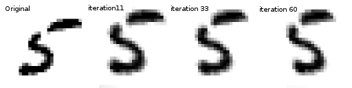
Visualizing the STN results

Now, we will inspect the results of our learned visual attention mechanism.

We define a small helper function in order to visualize the transformations while training.

def convert_image_np(inp):
    """Convert a Tensor to numpy image."""
    inp = inp.numpy().transpose((1, 2, 0))
    mean = np.array([0.485, 0.456, 0.406])
    std = np.array([0.229, 0.224, 0.225])
    inp = std * inp + mean
    inp = np.clip(inp, 0, 1)
    return inp

# We want to visualize the output of the spatial transformers layer
# after the training, we visualize a batch of input images and
# the corresponding transformed batch using STN.


def visualize_stn():
    with torch.no_grad():
        # Get a batch of training data
        data = next(iter(test_loader))[0].to(device)

        input_tensor = data.cpu()
        transformed_input_tensor = model.stn(data).cpu()

        in_grid = convert_image_np(
            torchvision.utils.make_grid(input_tensor))

        out_grid = convert_image_np(
            torchvision.utils.make_grid(transformed_input_tensor))

        # Plot the results side-by-side
        f, axarr = plt.subplots(1, 2)
        axarr[0].imshow(in_grid)
        axarr[0].set_title('Dataset Images')

        axarr[1].imshow(out_grid)
        axarr[1].set_title('Transformed Images')

for epoch in range(1, 20 + 1):
    train(epoch)
    test()

# Visualize the STN transformation on some input batch
visualize_stn()

plt.ioff()
plt.show()

/var/lib/ci-user/.local/lib/python3.10/site-packages/torch/nn/functional.py:5082: UserWarning:

Default grid_sample and affine_grid behavior has changed to align_corners=False since 1.3.0. Please specify align_corners=True if the old behavior is desired. See the documentation of grid_sample for details.

/var/lib/ci-user/.local/lib/python3.10/site-packages/torch/nn/functional.py:5015: UserWarning:

Default grid_sample and affine_grid behavior has changed to align_corners=False since 1.3.0. Please specify align_corners=True if the old behavior is desired. See the documentation of grid_sample for details.

Train Epoch: 1 [0/60000 (0%)]   Loss: 2.315653
Train Epoch: 1 [32000/60000 (53%)]      Loss: 1.036644
/var/lib/ci-user/.local/lib/python3.10/site-packages/torch/nn/_reduction.py:51: UserWarning:

size_average and reduce args will be deprecated, please use reduction='sum' instead.


Test set: Average loss: 0.2751, Accuracy: 9247/10000 (92%)

Train Epoch: 2 [0/60000 (0%)]   Loss: 0.591510
Train Epoch: 2 [32000/60000 (53%)]      Loss: 0.361250

Test set: Average loss: 0.2838, Accuracy: 9082/10000 (91%)

Train Epoch: 3 [0/60000 (0%)]   Loss: 0.688757
Train Epoch: 3 [32000/60000 (53%)]      Loss: 0.238103

Test set: Average loss: 0.1423, Accuracy: 9563/10000 (96%)

Train Epoch: 4 [0/60000 (0%)]   Loss: 0.391282
Train Epoch: 4 [32000/60000 (53%)]      Loss: 0.115492

Test set: Average loss: 0.1245, Accuracy: 9598/10000 (96%)

Train Epoch: 5 [0/60000 (0%)]   Loss: 0.215925
Train Epoch: 5 [32000/60000 (53%)]      Loss: 0.191664

Test set: Average loss: 0.1001, Accuracy: 9693/10000 (97%)

Train Epoch: 6 [0/60000 (0%)]   Loss: 0.122699
Train Epoch: 6 [32000/60000 (53%)]      Loss: 0.091529

Test set: Average loss: 0.0813, Accuracy: 9748/10000 (97%)

Train Epoch: 7 [0/60000 (0%)]   Loss: 0.127949
Train Epoch: 7 [32000/60000 (53%)]      Loss: 0.157717

Test set: Average loss: 0.0726, Accuracy: 9778/10000 (98%)

Train Epoch: 8 [0/60000 (0%)]   Loss: 0.318410
Train Epoch: 8 [32000/60000 (53%)]      Loss: 0.177054

Test set: Average loss: 0.0707, Accuracy: 9785/10000 (98%)

Train Epoch: 9 [0/60000 (0%)]   Loss: 0.088949
Train Epoch: 9 [32000/60000 (53%)]      Loss: 0.089132

Test set: Average loss: 0.0646, Accuracy: 9813/10000 (98%)

Train Epoch: 10 [0/60000 (0%)]  Loss: 0.093442
Train Epoch: 10 [32000/60000 (53%)]     Loss: 0.199287

Test set: Average loss: 0.0608, Accuracy: 9813/10000 (98%)

Train Epoch: 11 [0/60000 (0%)]  Loss: 0.155371
Train Epoch: 11 [32000/60000 (53%)]     Loss: 0.089858

Test set: Average loss: 0.0650, Accuracy: 9813/10000 (98%)

Train Epoch: 12 [0/60000 (0%)]  Loss: 0.114020
Train Epoch: 12 [32000/60000 (53%)]     Loss: 0.270379

Test set: Average loss: 0.0507, Accuracy: 9850/10000 (98%)

Train Epoch: 13 [0/60000 (0%)]  Loss: 0.101258
Train Epoch: 13 [32000/60000 (53%)]     Loss: 0.108374

Test set: Average loss: 0.0492, Accuracy: 9851/10000 (99%)

Train Epoch: 14 [0/60000 (0%)]  Loss: 0.074264
Train Epoch: 14 [32000/60000 (53%)]     Loss: 0.220129

Test set: Average loss: 0.0509, Accuracy: 9858/10000 (99%)

Train Epoch: 15 [0/60000 (0%)]  Loss: 0.057463
Train Epoch: 15 [32000/60000 (53%)]     Loss: 0.072608

Test set: Average loss: 0.0474, Accuracy: 9856/10000 (99%)

Train Epoch: 16 [0/60000 (0%)]  Loss: 0.056474
Train Epoch: 16 [32000/60000 (53%)]     Loss: 0.323527

Test set: Average loss: 0.0489, Accuracy: 9857/10000 (99%)

Train Epoch: 17 [0/60000 (0%)]  Loss: 0.266878
Train Epoch: 17 [32000/60000 (53%)]     Loss: 0.226094

Test set: Average loss: 0.0628, Accuracy: 9810/10000 (98%)

Train Epoch: 18 [0/60000 (0%)]  Loss: 0.021047
Train Epoch: 18 [32000/60000 (53%)]     Loss: 0.133307

Test set: Average loss: 0.0469, Accuracy: 9868/10000 (99%)

Train Epoch: 19 [0/60000 (0%)]  Loss: 0.081238
Train Epoch: 19 [32000/60000 (53%)]     Loss: 0.139788

Test set: Average loss: 0.0460, Accuracy: 9868/10000 (99%)

Train Epoch: 20 [0/60000 (0%)]  Loss: 0.089511
Train Epoch: 20 [32000/60000 (53%)]     Loss: 0.033778

Test set: Average loss: 0.0601, Accuracy: 9827/10000 (98%)